Point-scanning detectors
Open in Colab Download notebook
This tutorial compares a photomultiplier tube (PMT) and a hybrid detector (HyD)
on the same confocal image. It shows how the PMT high voltage trades signal
against clipping, and how photon counting and line averaging affect noise.
The complete script is
examples/point_detectors.py.
The confocal simulation
A single confocal plane of random lines labeled with EGFP, with 80 nm pixels:
from microsim import schema as ms
from microsim.schema.detectors import lib
from microsim.schema.optical_config.lib import LASER_488

sim = ms.Simulation(
    truth_space={"upscale": 4},
    output_space=ms.ShapeScaleSpace(shape=(1, 128, 128), scale=(0.16, 0.08, 0.08)),
    sample=[
        ms.FluorophoreDistribution(
            distribution=ms.MatsLines(density=0.5, length=30, azimuth=5, max_r=1),
            fluorophore="EGFP",
        )
    ],
    channels=[LASER_488.model_copy(update={"power": 2e4})],  # (1)!
    modality=ms.Confocal(pinhole_au=1),
    settings=ms.Settings(random_seed=100),
    detector=lib.HYD_SP8,  # (2)!
)
optical_image = sim.optical_image()
- A 488 nm laser with a 525/50 emission filter, at 20 kW/cm² at the focus (about 10 µW at 1.4 NA; the library default is 100 kW/cm²). The brightest pixels receive tens of millions of photons per second. EGFP is only slightly saturated at this irradiance (\(k\tau \approx 0.03\)).
- The detector's QE is applied when the optical image is computed. All the detectors compared below have GaAsP photocathodes with nearly identical QE spectra, so one optical image serves for all of them.
Four detector settings
digital_image accepts an existing optical image and an exposure time, so
each detector only repeats the last stage. For a point scanner, exposure_ms
is the pixel dwell time; here 1 µs.
import matplotlib.pyplot as plt

detectors = {
    "GaAsP PMT, 0.7 V": lib.PMT_GAASP.model_copy(update={"hv": 0.7}),
    "GaAsP PMT, 0.9 V": lib.PMT_GAASP.model_copy(update={"hv": 0.9}),
    "HyD (counting)": lib.HYD_SP8,
    "HyD, 4× averaging": lib.HYD_SP8.model_copy(update={"averaging": 4}),
}

fig, axes = plt.subplots(1, 4, figsize=(13, 3.8))
for ax, (name, detector) in zip(axes, detectors.items()):
    sim.detector = detector
    img = sim.digital_image(optical_image, exposure_ms=0.001)
    ax.imshow(img[0, 0], cmap="gray")
    ax.set_title(f"{name}\nmax gray value: {int(img.max())}")
    ax.axis("off")
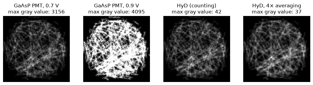
What to notice:
- PMT high voltage.
hvis the control voltage of a Hamamatsu photosensor module, 0.5–0.9 V. At 0.7 V the brightest pixels stay below the 12-bit maximum of 4095. At 0.9 V the gain is about 5 times higher, and many pixels clip. Raising the HV barely changes the signal-to-noise ratio of the photon signal, which is set by the number of photoelectrons; it scales the signal up relative to the amplifier noise and the digitization step. - Photon counting. The HyD reports photon counts directly (the maximum here is a few dozen), with no gain noise and no read noise. For the same photons its images are less noisy than the PMT's, mainly because the PMT's dynode gain is random (excess noise factor about 1.3).
- Averaging. With
averaging=4, each line is scanned four times and the counts are averaged. The brightness stays the same, and the noise falls by about a factor of 2.
Going further
The PMT model also includes output-current
saturation (max_output_current_ua, set in the library presets) and the
amplifier's time constant (time_constant_us), which smears signal along the
scan direction at short dwell times. The HyD model
includes count losses from dead time. See Detectors
for the details.