Detectors
The detector turns the optical image (photons per second at each pixel) into the digital image (integer gray values). This is where the exposure time enters, and where most of the noise comes from.
| Detector | camera_type |
Models |
|---|---|---|
CameraCCD |
"CCD" |
CCD cameras |
CameraEMCCD |
"EMCCD" |
electron-multiplying CCD cameras |
CameraCMOS |
"CMOS" |
CMOS and sCMOS cameras |
PMT |
"PMT" |
photomultiplier tubes, analog readout |
HyD |
"HyD" |
hybrid photodetectors, photon counting |
In dictionary form, camera_type selects the class:
detector={"camera_type": "EMCCD", "em_gain": 300}.
Without a detector
If detector is None (the default), the digital image is the expected
number of photons per pixel: the optical image times the exposure time,
binned to the output space, with no noise of any kind. Add a detector
to get shot noise.
A noise-free image (the ER of a HeLa cell, simulated by microsim) recorded by different cameras, all with QE = 1. The noise is drawn in your browser, with the same steps and distributions as microsim's detector model. At a few photons per pixel, the CCD's read noise dominates; the sCMOS is close to the shot-noise limit; the EMCCD's gain lifts single photons above its read noise, at the cost of extra gain noise.
Exposure time
Simulation.exposure_ms is the integration time per pixel, in milliseconds:
- for a camera, the exposure time of each frame;
- for a point scanner, the pixel dwell time (typically 0.0005–0.01 ms).
A channel can override it with
OpticalConfig.exposure_ms, and
digital_image(exposure_ms=...)
overrides both, which is a quick way to compare exposure times on one optical
image:
optical = sim.optical_image()
short = sim.digital_image(optical, exposure_ms=10)
long = sim.digital_image(optical, exposure_ms=1000)
The detector simulation pipeline
All detectors run the same sequence of steps. They differ in their parameters, and in which steps do nothing for them.
- Expected signal. Photons per second × integration time gives the mean number of photoelectrons per pixel. Dark current (and clock-induced charge, for cameras) is added.
- Shot noise. The number of photoelectrons is drawn from a Poisson distribution with that mean.
- Full well. A camera pixel cannot hold more than
full_wellelectrons. - Multiplication. EMCCDs and PMTs multiply each electron by a random gain before readout. The randomness adds noise.
- Readout. The amplifier adds Gaussian read noise, and the ADC converts
electrons to gray values, rounded and clipped to the top of the
bit_depthrange. Then any digital gain and theoffsetare applied, and the result is clipped to the range again.
The parameters shared by all detectors:
| Parameter | Meaning |
|---|---|
qe |
quantum efficiency, 0–1: a number, or a Spectrum over wavelength |
dark_current |
thermally generated electrons (or dark counts) per pixel per second |
read_noise |
electrons rms, added once per frame |
offset |
gray value added to every pixel |
bit_depth |
output gray values are clipped to 0 … 2bit_depth − 1 |
averaging |
number of frames (or scan passes) averaged into each image |
electrons_per_adu |
electrons per gray value, as on a camera datasheet |
relative_gain |
analog gain relative to the setting at which full_well maps to the maximum gray value (cameras only) |
Give either electrons_per_adu or relative_gain, not both. For cameras the
default is relative_gain=1, which maps a full pixel to the top of the ADC
range.
QE is applied in the optical image
The detector's qe is applied per wavelength when the emission rates are
computed (Photon budget), not in the
detector step. If you swap detectors on an existing optical image, the
new detector's QE is not used. Recompute the optical image, or compare
detectors with similar QE. See
#152.
Noise in more detail
Shot noise. Photons arrive at random, so the count in a pixel is Poisson distributed: its variance equals its mean \(n\), and the best possible signal-to-noise ratio is \(\sqrt{n}\).
Read noise \(\sigma_r\) is added once per readout, independent of the signal, so the SNR of a camera without gain is
Read noise dominates when \(n \lesssim \sigma_r^2\).
Excess noise. A random gain \(g\) per electron multiplies the variance by the excess noise factor \(F = \langle g^2 \rangle / \langle g \rangle^2\). After the gain, read noise is negligible but
so gain noise acts like dividing the QE by \(F\). microsim draws the multiplied signal from a gamma distribution with the right mean and variance. This is exact for an EMCCD at high gain, and approximate (in the shape of the distribution, not its mean or variance) at low gain.
Quantization. Rounding to integer gray values adds a uniform error of
variance 1/12 gray value². It matters when electrons_per_adu is large
compared with the read noise.
Averaging. With averaging=N, the signal and dark current are
integrated for N times the exposure, read noise is added N times, and the
result is divided by N. Brightness is unchanged, and noise is reduced.
SNR against signal
SNR of each camera, relative to an ideal detector that adds only shot noise, from the formulas above. Read noise matters at low signal; the EMCCD's gain removes it, at the cost of the excess noise factor, which caps its relative SNR at \(1/\sqrt{F} \approx 71\%\).
Cameras
CCD
CameraCCD: all pixels share one output
amplifier. Typical values: QE 0.5–0.7, read noise 5–10 e⁻, full well
15,000–20,000 e⁻.
EMCCD
CameraEMCCD adds an electron-multiplying
register before the amplifier. Each of its em_stages cells (604 by default)
multiplies the charge by a small random amount, for a mean gain em_gain
(typically 100–1000). The signal is lifted far above the read noise, so single
photons become detectable, but the excess noise factor rises toward 2: at high
gain an EMCCD has the SNR of a noise-free detector with half its QE.
Excess noise factor of the EM register,
CameraEMCCD.excess_noise_factor.
With an EMCCD, electrons_per_adu is usually easier to reason about than
relative_gain, because relative_gain refers to the pixel full well, before
the EM gain.
CMOS and sCMOS
CameraCMOS: each pixel has its own amplifier.
Typical values for a scientific CMOS: QE 0.7–0.95, read noise 1–2 e⁻,
electrons_per_adu around 0.5 at 16 bits.
sCMOS pixel-to-pixel variation is not modeled
The model applies the same gain, offset, and read noise to every pixel. Real sCMOS sensors vary from pixel to pixel, and some pixels are much noisier than average, so simulated sCMOS images are more uniform than real ones. Per-pixel gain, offset, and read noise maps are on the roadmap.
Default camera settings
All cameras default to QE 1, read noise 6 e⁻, full well 18,000 e⁻, 12 bits,
offset 100, and dark current 0.001 e⁻/pixel/s. These are not meant to
match any particular camera. Set the values from your camera's datasheet,
or start from the library model lib.ICX285.
Point detectors
A point scanner records one pixel at a time, so its detectors have no pixels
to hold charge, no full well, and no relative_gain. Set their gain with
electrons_per_adu, or the parameters below. exposure_ms is the pixel dwell
time.
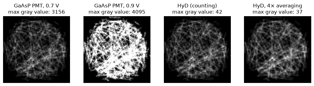
The same confocal optical image, recorded with 1 µs pixel dwell by a GaAsP PMT at two control voltages and by a HyD in photon-counting mode, without and with 4× averaging. At 0.9 V many PMT pixels clip at the top of the 12-bit range. The HyD gives raw photon counts. From the point-scanning detectors tutorial.
PMT
PMT models a photomultiplier tube read out in analog
mode. A photoelectron from the photocathode is multiplied by a chain of
dynodes, and the resulting current is integrated over the dwell time.
- Gain. Set the high voltage
hvas on the microscope. The gain follows a power law,ref_gain × (hv / ref_hv) ** hv_exponent. The defaults model a Hamamatsu GaAsP photosensor module controlled by a 0.5–0.9 V signal, with a gain of 5 × 10⁵ at 0.8 V. To set the gain directly, usehv_gaininstead. - Gain noise. The excess noise factor follows from the gain per dynode, and increases as the HV is lowered (about 1.3 at 0.9 V, 1.5 at 0.5 V for the default tube).
- Digital gain.
digital_gainmultiplies the digitized signal, like the digital gain setting in some acquisition software. It amplifies signal and noise equally. - Saturation. If
max_output_current_uais set, the gain drops as the average anode current approaches that limit. The current is averaged overdivider_time_constant_msalong the scan, so a bright region dims itself and the lines that follow it. - Amplifier bandwidth. If
time_constant_us> 0, the signal of each pixel leaks into the next few pixels along X, producing a streak at short dwell times.
Gain and excess noise factor of the PMT presets in
detectors.lib across their control voltage range.
HyD
HyD models a hybrid photodetector (as in Leica HyD
detectors) in photon-counting mode. Every photon gives nearly the same pulse,
so pulses are counted: no gain noise and no read noise. With the default
electrons_per_adu=1, the output is the photon count.
After each pulse the detector is blind for dead_time_ns (1.5 ns by
default), so at high count rates some photons are missed: a true rate \(n\) is
recorded as \(n / (1 + n\tau)\), about 6% low at 40 million counts per second.
Dead time also makes the counts more regular than Poisson.
Fraction of photons counted by a photon counter with a non-paralyzable dead time, against the true photon rate.
Detector library
microsim.schema.detectors.lib has
detectors with published or measured parameters:
| Name | Type | Notes |
|---|---|---|
ICX285 |
CCD | Sony ICX285 sensor, with its QE spectrum |
PMT_GAASP |
PMT | GaAsP photocathode, QE spectrum from FPbase, 2 µA max. output |
PMT_MULTIALKALI |
PMT | multialkali photocathode, QE 0.2, 100 µA max. output |
HYD_SP8 |
HyD | GaAsP hybrid detector |
POWER_HYD_R |
HyD | red-extended GaAsP hybrid detector |
The source code of
detectors/lib.py
lists where each value comes from.
The detector docstrings in the API reference describe each model in more detail, including what is not modeled.