Overview
A microsim simulation follows the light from the sample to the detector. This page describes the parts of a simulation and the order in which they are used. The following pages cover each part in detail.
The Simulation object
All parameters live on one Simulation object. Its
fields map onto parts of a real experiment:
| Field | What it describes | Guide |
|---|---|---|
truth_space |
the grid on which the sample and optics are computed | Spaces |
output_space |
the pixel grid of the final image | Spaces |
sample |
where the fluorophores are, and which fluorophores they are | Samples |
channels |
light sources and filters, one entry per channel | Channels |
tracks |
which channels are acquired at the same time | Channels |
objective_lens |
numerical aperture, refractive indices, coverslip | Modalities |
modality |
how the image is formed: widefield, confocal, ... | Modalities |
detector |
camera or point detector, and its noise | Detectors |
exposure_ms |
camera exposure, or pixel dwell time for point scanners | Detectors |
settings |
compute backend, precision, random seed, caching | Settings |
output_path |
where to save the result | Saving and loading |
Only truth_space and sample are required.
The stages
Simulation.run() computes four things in order.
Each is also available as a method, so you can stop at any stage, inspect the
intermediate result, or change a parameter and repeat only the later stages.
flowchart TB
    subgraph S1 ["<span class='ms-stage'>1</span> ground_truth()"]
      direction LR
      sp[truth_space] --> gt["fluorophores per voxel<br/><code>(f, z, y, x)</code>"]
      sa[sample] --> gt
    end
    subgraph S2 ["<span class='ms-stage'>2</span> filtered_emission_rates()"]
      direction LR
      fl[fluorophore spectra] --> em["photons/s per fluorophore<br/><code>(c, f, w)</code>"]
      ch["channels, tracks"] --> em
      ob1[objective NA, specimen RI] --> em
      dq[detector QE] --> em
    end
    subgraph S3 ["<span class='ms-stage'>3</span> optical_image()"]
      direction LR
      mo[modality + objective → PSF] --> oi["photons/s per voxel<br/><code>(c, z, y, x)</code>"]
    end
    subgraph S4 ["<span class='ms-stage'>4</span> digital_image()"]
      direction LR
      os[output_space] --> di["gray values<br/><code>(c, z, y, x)</code>"]
      de[detector + exposure] --> di
    end
    S1 --> S3
    S2 --> S3
    S3 --> S4
1 Ground truth. Each label in the sample is
drawn into the truth space. The result counts fluorophores per voxel, with one
layer per label (f). See Samples.
2 Emission rates. For every pair of
fluorophore and channel, microsim computes how many photons per second one
fluorophore emits and how many reach the detector, as a function of wavelength
(w). This includes the light source, excitation and emission filters, the
fluorophore's absorption and emission spectra, extinction coefficient and
quantum yield, the fraction of light the objective collects, and the
detector's quantum efficiency. It has no spatial dimensions. Because every
fluorophore is computed in every channel, bleedthrough and cross-excitation
follow automatically. Channels acquired at the same time (tracks) excite
the sample together. See Channels and
Photon budget.
3 Optical image. The ground truth of each fluorophore is multiplied by its emission rate and convolved with the microscope's point spread function (PSF), then the fluorophores are summed within each channel. The result is the noise-free light distribution at the detector, in photons per second, still on the truth-space grid. See Modalities.
4 Digital image. The optical image is binned to the output space, multiplied by the exposure time, and passed through the detector model, which adds shot noise, dark current, gain, read noise, and digitization. See Detectors.
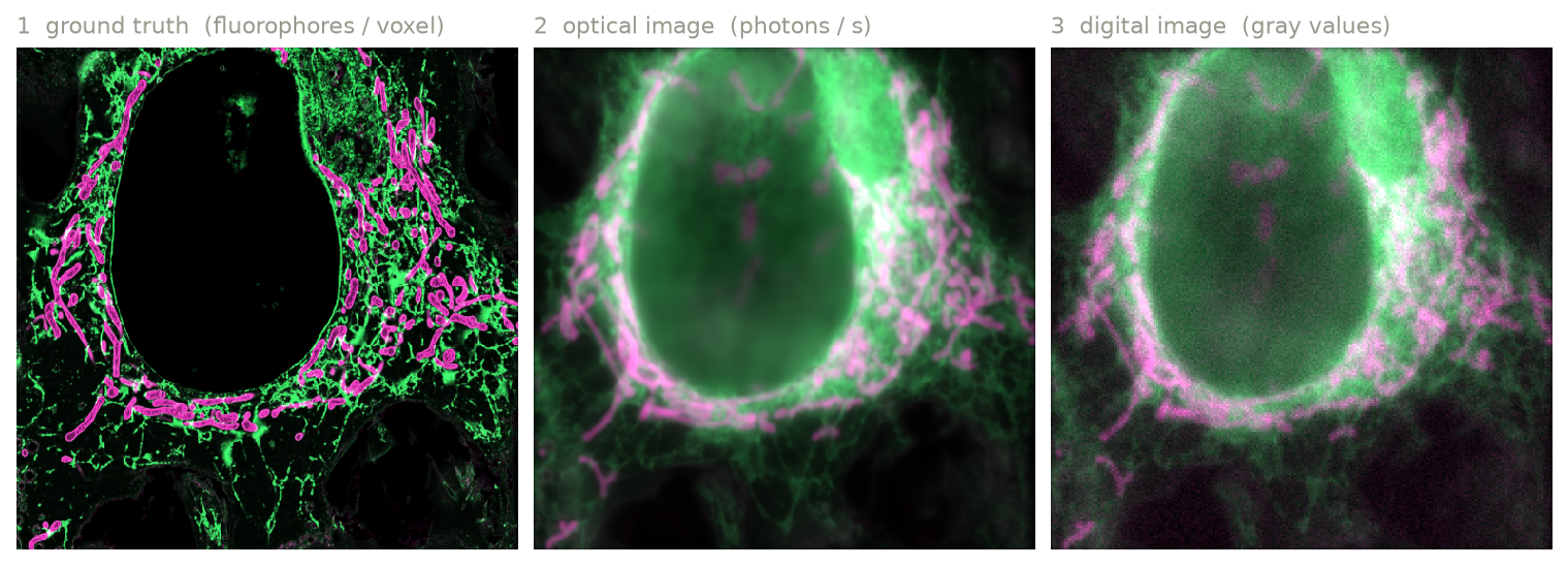
Ground truth (left), optical image (center), and digital image (right) for endoplasmic reticulum labeled with EGFP (green) and mitochondria labeled with mCherry (magenta). The ground truth is from OpenOrganelle; see the two-color tutorial.
There are two more methods for analysis.
optical_image_per_fluor()
returns the optical image before fluorophores are summed, as
(c, f, z, y, x), which shows how much of each channel comes from each
fluorophore. emission_flux() returns the
emitted photons per voxel before blurring.
To simulate many samples with the same optics,
run_batch() runs the
simulation once per sample and yields each digital image. PSFs and emission
rates are computed once and reused. Each sample gets its own random seed,
derived from settings.random_seed, and if output_path is set, result i
is written to <stem>_<i>.<suffix>.
Units
microsim uses one unit per kind of quantity:
| Quantity | Unit |
|---|---|
| lengths (space scale, extent) | µm |
| wavelengths | nm |
irradiance (power) |
W/cm² |
| exposure and dwell time | ms |
| extinction coefficient | M⁻¹ cm⁻¹ |
| fluorescence lifetime | ns |
Outputs are labeled arrays
Every stage returns an xarray.DataArray. Its dimensions
have names, and z, y, x carry coordinates in µm, so you can select and
reduce by name:
digital = sim.run()
digital.sel(c="FITC")  # select a channel by name
digital.isel(z=8).plot()  # plot a plane (needs matplotlib)
sim.ground_truth().max("z")  # maximum projection
Use digital.values (or numpy.asarray(digital)) for a plain NumPy array.
With a GPU backend, digital.data is a GPU array; see
Settings.
What is (and isn't) modeled
microsim aims to make each modeled step physically correct, and to state the approximations. The guide pages list the details for each part. In summary, these are not modeled at present:
- photobleaching, blinking, and other time-dependent fluorophore behavior (emission is a steady-state rate)
- triplet and other dark states, and stimulated emission
- scattering, absorption, and aberrations from the sample (other than the refractive index mismatch handled by the PSF model)
- out-of-focus background other than what the PSF produces, and autofluorescence
- pixel-to-pixel variation of sCMOS cameras
- the camera's physical pixel size and magnification (the output pixel size
is set by
output_space)